PlasmonDispersion

graphenemodeling.graphene.monolayer.PlasmonDispersion(q, gamma, FermiLevel, eps1, eps2, T, model)

Returns the nonretarded plasmon dispersion relations E(q) for a surface plasmon in an infinite sheet of graphene sandwiched between two dielectrics eps1 and eps2.

All values returned are assumed to be at zero temperature with no loss (gamma).

Parameters:

• q (array-like, rad/m) – Wavenumber of the plasmon
• eps1 (scalar, unitless) – Permittivity in upper half-space
• eps2 (scalar, unitless) – Permittivity in lower half-space
• model (string) – ‘intra’ for intraband dispersion, ‘local’ uses the intraband + interband constributions to the conductivity, and ‘nonlocal’ for fully nonlocal conductivity.

Returns:

omega – Frequency of the plasmon with wavenumber q

Return type:

array-like

Notes

model=='intra' uses

\[\omega = \frac{1}{\hbar}\sqrt{\frac{e^2\epsilon_F}{2\pi\epsilon_0\bar\epsilon}q}\]

model=='local' uses

\[1-\frac{i\text{Im}[\sigma(q,\omega)]}{2i\epsilon_0\bar\epsilon\omega}=0\]

and finally, model=='nonlocal' uses

\[1 - \frac{\sigma(q,\omega)q}{2i\epsilon_0\bar\epsilon\omega} = 0\]

Examples

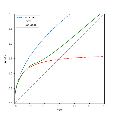
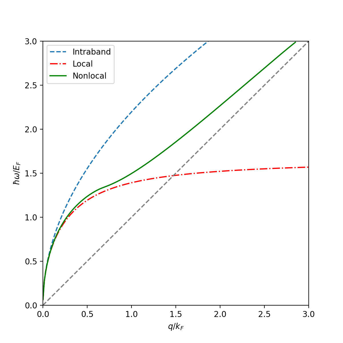
Plot the three expressions for the dispersion relation. Replicates Fig. 5.2 in Ref. [1].

>>> from graphenemodeling.graphene import monolayer as mlg
>>> from scipy.constants import elementary_charge, hbar
>>> eV = elementary_charge
>>> gamma=0.012 * eV / hbar
>>> eF = 0.4*eV
>>> kF = mlg.FermiWavenumber(eF,model='LowEnergy')
>>> q = np.linspace(1e-3,3,num=200) * kF
>>> disp_intra = mlg.PlasmonDispersion(q,gamma,eF,eps1=1,eps2=1,T=0,model='intra')
>>> disp_local = mlg.PlasmonDispersion(q,gamma,eF,eps1=1,eps2=1,T=0,model='local')
>>> disp_nonlocal = mlg.PlasmonDispersion(q,gamma,eF,eps1=1,eps2=1,T=0,model='nonlocal')
>>> fig, ax = plt.subplots(figsize=(6,6))
>>> ax.plot(q/kF,hbar*disp_intra/eF,'--',label='Intraband')
<...
>>> ax.plot(q/kF,hbar*disp_local/eF,'r-.',label='Local')
<...
>>> ax.plot(q[:190]/kF,hbar*disp_nonlocal[:190]/eF,'g',label='Nonlocal')
<...
>>> ax.plot(q/kF,q/kF,color='gray',linestyle='--')
<...
>>> ax.set_xlabel('$q/k_F$')
>>> ax.set_ylabel('$\hbar\omega/E_F$')
>>> ax.set_xlim(0,3)
>>> ax.set_ylim(0,3)
>>> plt.legend()
>>> plt.show()

(Source code, png, hires.png, pdf)

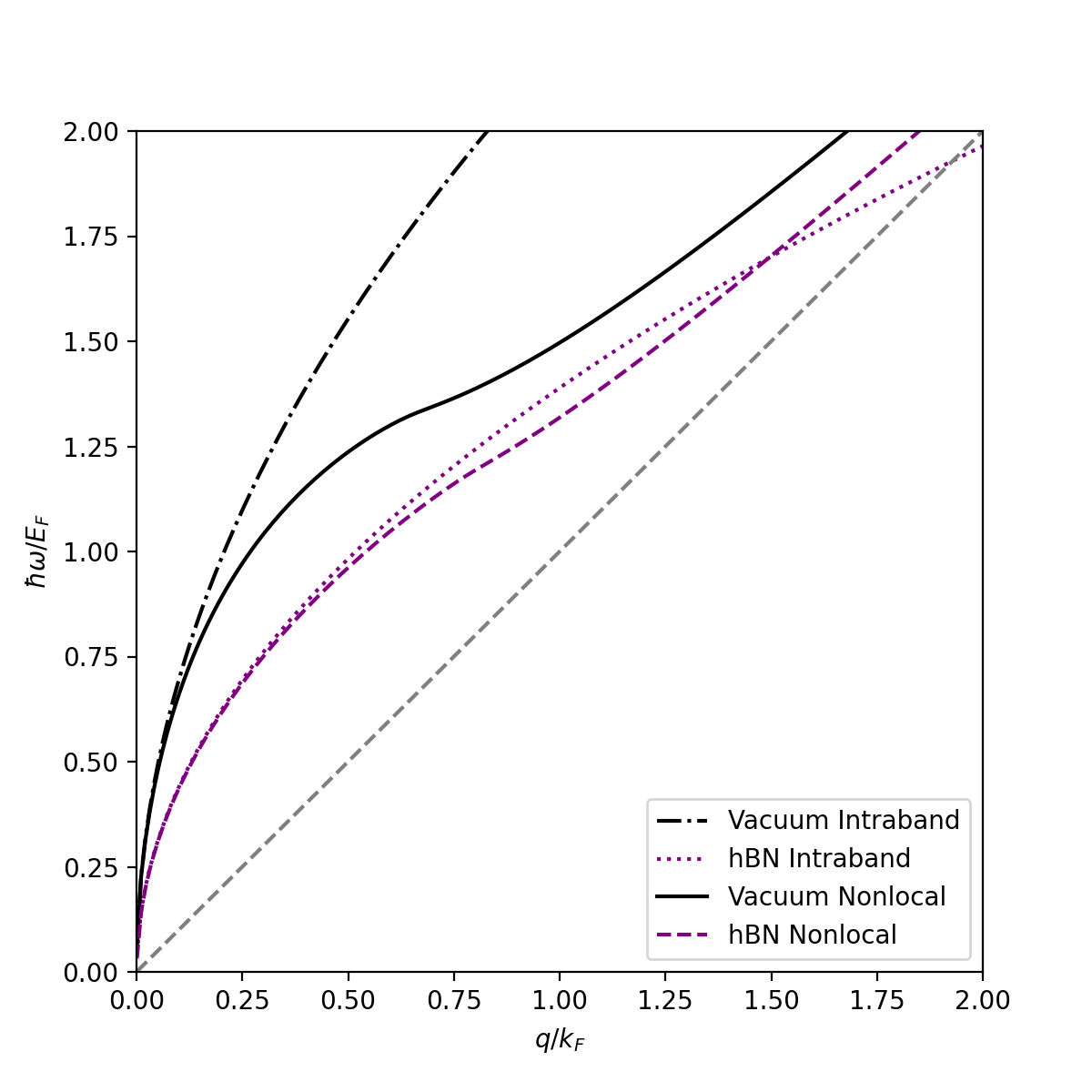
Plot dispersion relation with a lower half-space permittivity of \(\epsilon=4\) (an approximation for hexagonal boron nitride). Replicates Fig. 1d in Ref. [2].

>>> from graphenemodeling.graphene import monolayer as mlg
>>> from scipy.constants import elementary_charge, hbar
>>> eV = elementary_charge
>>> gamma=0.012 * eV / hbar
>>> eF = 0.4*eV
>>> kF = mlg.FermiWavenumber(eF,model='LowEnergy')
>>> q = np.linspace(1e-3,2,num=200) * kF
>>> vac_intra = mlg.PlasmonDispersion(q,gamma,eF,eps1=1,eps2=1,T=0,model='intra')
>>> hbn_intra = mlg.PlasmonDispersion(q,gamma,eF,eps1=1,eps2=4,T=0,model='intra')
>>> vac_nonlocal = mlg.PlasmonDispersion(q,gamma,eF,eps1=1,eps2=1,T=0,model='nonlocal')
>>> hbn_nonlocal = mlg.PlasmonDispersion(q,gamma,eF,eps1=1,eps2=4,T=0,model='nonlocal')
>>> fig, ax = plt.subplots(figsize=(6,6))
>>> ax.plot(q/kF,hbar*vac_intra/eF,'k-.',label='Vacuum Intraband')
<...
>>> ax.plot(q/kF,hbar*hbn_intra/eF,linestyle='dotted',color='purple',label='hBN Intraband')
<...
>>> ax.plot(q/kF,hbar*vac_nonlocal/eF,'k-',label='Vacuum Nonlocal')
<...
>>> ax.plot(q/kF,hbar*hbn_nonlocal/eF,'--',color='purple',label='hBN Nonlocal')
<...
>>> ax.plot(q/kF,q/kF,color='gray',linestyle='--')
<...
>>> ax.set_xlabel('$q/k_F$')
>>> ax.set_ylabel('$\hbar\omega/E_F$')
>>> ax.set_xlim(0,2)
>>> ax.set_ylim(0,2)
>>> plt.legend()
>>> plt.show()

(Source code, png, hires.png, pdf)

References

[1] Christensen, T. (2017). From Classical to Quantum Plasmonics in Three and Two Dimensions (Cham: Springer International Publishing). http://link.springer.com/10.1007/978-3-319-48562-1.

[2] Jablan, M., Buljan, H., and Soljačić, M. (2009). Plasmonics in graphene at infrared frequencies. Phys. Rev. B 80, 245435. https://link.aps.org/doi/10.1103/PhysRevB.80.245435.