ScalarOpticalConductivity

graphenemodeling.graphene.monolayer.ScalarOpticalConductivity(q, omega, gamma, FermiLevel, T, model=None)

The diagonal conductivity of graphene \(\sigma_{xx}\).

Parameters:

• q (array-like, rad/m) – Wavenumber
• omega (array-like, rad/s) – Angular frequency
• FermiLevel (scalar, J) – the Fermi energy
• gamma (scalar, rad/s) – scattering rate
• T (scalar, K) – Temperature
• model (string) – Typically ‘None’, but for a specific model, specify it.

Returns:

• array-like
• conductivity at every value of omega

Examples

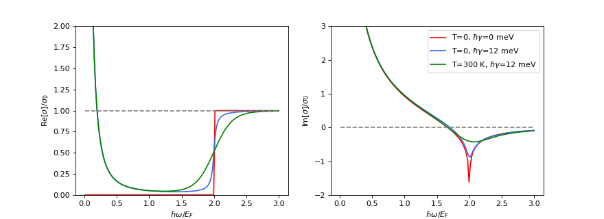
Plot the optical conductivity normalized to intrinsic conductivity \(\sigma_0\). Replicates Fig. 4.4 in Ref. [1].

>>> from graphenemodeling.graphene import monolayer as mlg
>>> from scipy.constants import elementary_charge, hbar
>>> from graphenemodeling.graphene._constants import sigma_0
>>> import matplotlib.pyplot as plt
>>> eF = 0.4 * elementary_charge
>>> g = 0.012 * elementary_charge / hbar
>>> w = np.linspace(0.01,3,num=150) / (hbar/eF)
>>> s_0K_0g = mlg.ScalarOpticalConductivity(q=0,omega=w,gamma=0,FermiLevel=eF,T=0)
>>> s_0K_12g = mlg.ScalarOpticalConductivity(q=0,omega=w,gamma=g,FermiLevel=eF,T=0.01)
>>> s_300K_12g = mlg.ScalarOpticalConductivity(q=0,omega=w,gamma=g,FermiLevel=eF,T=300)
>>> fig, (re_ax, im_ax) = plt.subplots(1,2,figsize=(11,4))
>>> s_Re = np.real(s_0K_0g)
>>> s_Im = np.imag(s_0K_0g)
>>> re_ax.plot(w*hbar/eF,s_Re/sigma_0,'r',label='T=0, $\hbar\gamma$=0 meV')
<...
>>> im_ax.plot(w*hbar/eF,s_Im/sigma_0,'r',label='T=0, $\hbar\gamma$=0 meV')
<...
>>> s_Re = np.real(s_0K_12g)
>>> s_Im = np.imag(s_0K_12g)
>>> re_ax.plot(w*hbar/eF,s_Re/sigma_0,color='royalblue',label='T=0, $\hbar\gamma$=12 meV')
<...
>>> im_ax.plot(w*hbar/eF,s_Im/sigma_0,color='royalblue',label='T=0, $\hbar\gamma$=12 meV')
<...
>>> s_Re = np.real(s_300K_12g)
>>> s_Im = np.imag(s_300K_12g)
>>> re_ax.plot(w*hbar/eF,s_Re/sigma_0,color='green',label='T=300 K, $\hbar\gamma$=12 meV')
<...
>>> im_ax.plot(w*hbar/eF,s_Im/sigma_0,color='green',label='T=300 K, $\hbar\gamma$=12 meV')
<...
>>> re_ax.set_ylabel('Re[$\sigma$]/$\sigma_0$')
>>> re_ax.set_xlabel('$\hbar\omega/E_F$')
>>> re_ax.plot(w*hbar/eF,np.ones_like(w),'--',color='gray')
>>> re_ax.set_ylim(0,2)
>>> im_ax.set_ylabel('Im[$\sigma$]/$\sigma_0$')
>>> im_ax.set_xlabel('$\hbar\omega/E_F$')
>>> im_ax.plot(w*hbar/eF,np.zeros_like(w),'--',color='gray')
>>> im_ax.set_ylim(-2,3)
>>> plt.legend()
>>> plt.show()

(Source code, png, hires.png, pdf)

Notes

The matrix optical conductivity \(\overleftrightarrow{\sigma}(q,\omega)\) relates the surface current \(\mathbf K(\omega)\) to an applied electric field \(\mathbf E(\omega)\). The fully general, anisotropic, nonlocal expression is given by

\[\mathbf K(\omega)=\int \overleftrightarrow\sigma(q,\omega)\mathbf E(\omega) dq\]

Here, \(\omega\) refers to the frequency and \(q\) refers to the scattering wavevector. The above expression fully general incorporating anisotropies and nonlocality and is rarely needed. In most cases, \(\overleftrightarrow{\sigma}\) is isotropic, so the above equation can be reduced to a scalar equation

\[K(\omega)=\int \sigma(q,\omega)E(\omega)dq\]

This is the conductivity in this function. The most general expression for the conductivity is given by the Kubo formula

\[\sigma(q,\omega)=\frac{ie^2\omega}{q^2}\chi^0(q,\omega).\]

where \(\chi^0\) is the Polarizibility. If q is nonzero, this form is used. However, it is common to use a simpler limiting cases of this expression. The local conductivity (called when q==0) is the one which is most familiar and it relates the surface current to the electric field linearly

\[\mathbf K(\omega)=\sigma(\omega)\mathbf E\]

It can be found from the nonlocal conductivity by taking the limit \(\lim_{q\to 0}\sigma(q,\omega)=\sigma(\omega)\) and takes the form \(\sigma(\omega)=\sigma_{intra}(\omega)+\sigma_{inter}(\omega)\), where the intraband and interband components are given by

\[\sigma_{intra}(\omega) = \frac{2ie^2k_BT}{\pi\hbar^2(\omega+i\gamma)}\ln\left [ 2 \cosh \frac{E_F}{2k_BT} \right ]\]

and

\[\sigma_{inter}(\omega) = \frac{e^2}{4\hbar}\left [ H(\hbar\omega/2) + \frac{4i}{\pi}\hbar ( \omega +i \gamma )\int_0^\infty \frac{H( \epsilon )-H(\hbar\omega /2)}{\hbar^2(\omega +i\gamma )^2-4\epsilon^2} d\epsilon\right ]\]

where

\[H(\epsilon) = f(-\epsilon)-f(\epsilon) = \frac{\sinh(\epsilon/k_BT)}{\cosh(E_F/k_BT) + \cosh(\epsilon/k_BT)}\]

For T=0 these expressions reduce to

\[\sigma_{intra}(\omega) = \frac{ie^2E_F}{\pi\hbar^2(\omega+i\gamma)}\]

\[\sigma_{inter}(\omega) = \frac{e^2}{4\hbar}\left [ \Theta(\hbar\omega - 2E_F) + \frac{i}{\pi} \ln\left [\frac{2E_F-\hbar\omega}{2E_F+\hbar\omega} \right ] \right ]\]

References

[1] Christensen, T. (2017). From Classical to Quantum Plasmonics in Three and Two Dimensions (Cham: Springer International Publishing). http://link.springer.com/10.1007/978-3-319-48562-1