DensityOfStates

graphenemodeling.graphene.monolayer.DensityOfStates(E, model, g0prime=0.0)

The density of states per square meter of graphene at energy \(E\).

Parameters:

• E (array-like, J) – Energy \(E\) at which to evaluate density of states.
• model (string) – 'LowEnergy'``or ``'FullTightBinding'
• g0prime (scalar, J) – The particle-hole asymmetry parameter \(\gamma_0'\). Typically \(0.02\gamma_0\leq\gamma_0'\leq 0.2\gamma_0\).

Returns:

Density of states, units are states per J-m^2

Return type:

array-like

Notes

For model==LowEnergy, the form is simply

\[\rho(E)=\frac{2}{\pi}\frac{|E|}{\hbar^2 v_F^2}\]

whereas the FullTightBinding model has a much more complicated form (eqn. 14 of [2])

\[\rho(E)=\frac{4}{\pi^2}\frac{|E|}{\gamma_0^2}\frac{1}{\sqrt{Z_0}}\mathbf{F}\left(\frac{\pi}{2},\sqrt{\frac{Z_1}{Z_0}}\right)\]

where \(\mathbf{F}(\pi/2,x)\) is the complete elliptic integral of the first kind (see scipy.special.ellipk) and

\[ \begin{align}\begin{aligned}Z_0 = \left\{\array{ (1 + |E/\gamma_0|)^2 - \frac{[(E/\gamma_0)^2-1]^2}{4}, & |E|\leq \gamma_0\\ 4|E/\gamma_0|, & -3\gamma_0\leq E \leq -\gamma_0,\gamma_0\leq E\leq 3\gamma_0 }\right.\\Z_1 = \left\{\array{ 4|E/\gamma_0|, & |E|\leq \gamma_0\\ (1 + |E/\gamma_0|)^2 - \frac{[(E/\gamma_0)^2-1]^2}{4}, & -3\gamma_0\leq E \leq -\gamma_0,\gamma_0\leq E\leq 3\gamma_0 }\right.\end{aligned}\end{align} \]

Examples

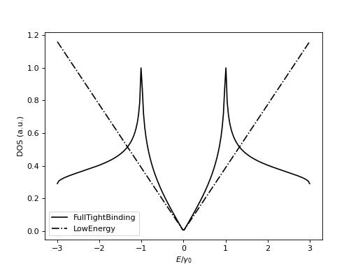
Plot the density of states for model=LowEnergy approximation and model=FullTightBinding model. Replicates Fig. 5 in Ref. [2].

>>> from graphenemodeling.graphene import monolayer as mlg
>>> from graphenemodeling.graphene import _constants as _c
>>> import matplotlib.pyplot as plt
>>> E = np.linspace(-3,3,num=200) * _c.g0
>>> DOS_low = mlg.DensityOfStates(E,model='LowEnergy')
>>> DOS_full = mlg.DensityOfStates(E,model='FullTightBinding')
>>> plt.plot(E/_c.g0,DOS_full/np.max(DOS_full),'k-',label='FullTightBinding')
[<...
>>> plt.plot(E/_c.g0,DOS_low/np.max(DOS_full),'k-.',label='LowEnergy')
[<...
>>> plt.xlabel('$E/\gamma_0$')
Text...
>>> plt.ylabel('DOS (a.u.)')
Text...
>>> plt.legend()
<...
>>> plt.show()

(Source code, png, hires.png, pdf)

References

[1] Hobson, J.P., and Nierenberg, W.A. (1953). The Statistics of a Two-Dimensional, Hexagonal Net. Phys. Rev. 89, 662–662. https://link.aps.org/doi/10.1103/PhysRev.89.662.

[2] Castro Neto, A.H., Guinea, F., Peres, N.M.R., Novoselov, K.S., and Geim, A.K. (2009). The electronic properties of graphene. Rev. Mod. Phys. 81, 109–162. https://link.aps.org/doi/10.1103/RevModPhys.81.109.