CarrierDispersion

graphenemodeling.graphene.monolayer.CarrierDispersion(k, model, eh=1, g0prime=0.0)

The dispersion of Dirac fermions in monolayer graphene.

These are the eigenvalues of the Hamiltonian. However, in both the LowEnergy model and the FullTightBinding model, we use closed form solutions rather than solving for the eigenvalues directly. This saves time and make broadcasting easier.

Parameters:

• k (array-like, complex, rad/m) – Wavevector of Dirac fermion relative to K vector. For 2D wavevectors, use \(k= k_x + i k_y\).
• model (string) –

  'LowEnergy': Linear approximation of dispersion.

  'FullTightBinding': Eigenvalues of tight-binding approximation. We use a closed form rather than finding eigenvalues of Hamiltonian to save time and avoid broadcasting issues.

• eh (int) – Band index: eh=1 returns conduction band, eh=-1 returns valence band

Returns:

dispersion – Dispersion relation evaluated at k.

Return type:

complex ndarray

Raises:

• ValueError – if model is not ‘LowEnergy’ or ‘FullTightBinding’.
• ValueError – if eh not 1 or -1.

Notes

When model='LowEnergy',

\[E =\pm\hbar v_F |k|\]

When model=FullTightBinding,

\[E = \pm \gamma_0 \sqrt{3 + f(k)} - \gamma_0'f(k)\]

where \(f(k)= 2 \cos(\sqrt{3}k_y a) + 4 \cos(\sqrt{3}k_y a/2)\cos(3k_xa/2)\).

Both expressions are equivalent to diagonalizing the Hamiltonian of the corresponding model.

Examples

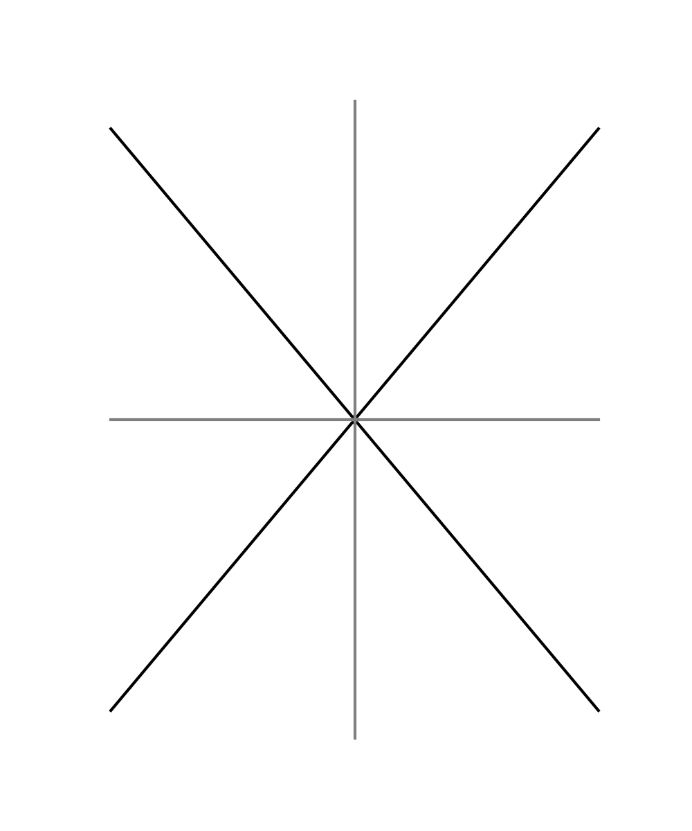
Plot the Fermion dispersion relation.

>>> import matplotlib.pyplot as plt
>>> from graphenemodeling.graphene import monolayer as mlg
>>> from scipy.constants import elementary_charge as eV
>>> eF = 0.4*eV
>>> kF = mlg.FermiWavenumber(eF,model='LowEnergy')
>>> k = np.linspace(-2*kF,2*kF,num=100)
>>> conduction_band = mlg.CarrierDispersion(k,model='LowEnergy')
>>> valence_band = mlg.CarrierDispersion(k,model='LowEnergy',eh=-1)
>>> fig, ax = plt.subplots(figsize=(5,6))
>>> ax.plot(k/kF,conduction_band/eF,'k')
[...
>>> ax.plot(k/kF,valence_band/eF, 'k')
[...
>>> ax.plot(k/kF,np.zeros_like(k),color='gray')
[...
>>> ax.axvline(x=0,ymin=0,ymax=1,color='gray')
<...
>>> ax.set_axis_off()
>>> plt.show()

(Source code, png, hires.png, pdf)

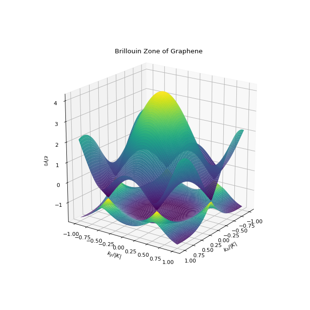
Plot the full multi-dimensional dispersion relation with a particle-hole asymmetry. Replicates Figure 3 in Ref. [1].

>>> from graphenemodeling.graphene import monolayer as mlg
>>> from graphenemodeling.graphene import _constants as _c
>>> import matplotlib.pyplot as plt
>>> from mpl_toolkits import mplot3d # 3D plotting
>>> kmax = np.abs(_c.K)
>>> emax = mlg.CarrierDispersion(0,model='FullTightBinding',g0prime=-0.2*_c.g0)
>>> kx = np.linspace(-kmax,kmax,num=100)
>>> ky = np.copy(kx)
>>> k = (kx + 1j*ky[:,np.newaxis]) + _c.K # k is relative to K. Add K to move to center of Brillouin zone
>>> conduction_band = mlg.CarrierDispersion(k,model='FullTightBinding',eh=1,g0prime=-0.2*_c.g0)
>>> valence_band = mlg.CarrierDispersion(k,model='FullTightBinding',eh=-1,g0prime=-0.2*_c.g0)
>>> fig = plt.figure(figsize=(8,8))
>>> fullax = plt.axes(projection='3d')
>>> fullax.view_init(20,35)
>>> KX, KY = np.meshgrid(kx,ky)
>>> fullax.plot_surface(KX/kmax,KY/kmax,conduction_band/_c.g0,rstride=1,cstride=1,cmap='viridis',edgecolor='none')
<...
>>> fullax.plot_surface(KX/kmax,KY/kmax,valence_band/_c.g0,rstride=1,cstride=1,cmap='viridis',edgecolor='none')
<...
>>> fullax.set_xlabel('$k_x/|K|$')
Text...
>>> fullax.set_ylabel('$k_y/|K|$')
Text...
>>> fullax.set_zlabel('$\epsilon/\gamma_0$')
Text...
>>> fullax.set_title('Brillouin Zone of Graphene')
Text...
>>> plt.show()

(Source code, png, hires.png, pdf)

References

[1] Wallace, P.R. (1947). The Band Theory of Graphite. Phys. Rev. 71, 622–634. https://link.aps.org/doi/10.1103/PhysRev.71.622

[1] Slonczewski, J.C., and Weiss, P.R. (1958). Band Structure of Graphite. Phys. Rev. 109, 272–279. https://link.aps.org/doi/10.1103/PhysRev.109.272.

[2] Falkovsky, L.A., and Varlamov, A.A. (2007). Space-time dispersion of graphene conductivity. Eur. Phys. J. B 56, 281–284. https://link.springer.com/article/10.1140/epjb/e2007-00142-3.

[4] Castro Neto, A.H., Guinea, F., Peres, N.M.R., Novoselov, K.S., and Geim, A.K. (2009). The electronic properties of graphene. Rev. Mod. Phys. 81, 109–162. https://link.aps.org/doi/10.1103/RevModPhys.81.109.